The old Fisher and the sea

---

The density function from probability theory does not describe the probability that an event occurs. It is obvious, but is nice to be reminded of it regularily. An event in that sense is the occurence, the realisation of e.g. a value x from a continuously defined random variable X. Only through the integration over a region or interval a < x < b where that specific event might occur, a statement about that occurrence happening in form of probability can be calculated. The most famous probability density function is maybe the normal distribution from Gauss. A lot of phenomens in nature and engineering can be approximated by that distribution. Often times in statistics classes, the distribution parameters are known beforehand. In real life, one could make the assumption, that the phenomena is is Gaussian distributed but the parameters are not known. It has two parameters μ and σ as shown by two different σ in figure 1. A large one (green) and a small one (blue) widens and stretches the distribution.

Intuitively, a sample from a distribution in figure 1 with a small variance will be close to the mean, hence it would deliver more information about the mean than a distribution's sample with the same mean but a very high variance. Meaning, once you measure once a phenomena from a distribution with a low variance, the actual sample would be close to the mean. It has to be, because the variance is low. It would be very unlikely to have measured a sample that it is not close to the mean. Doing some measurements, the average of those would be close to the mean. Hence those samples deliver more information about the mean. The Fisher information is a term that describes that idea and it gives a scalar value about the amout of information a sample from a distribution delivers about its distribution parameters. The Fisher information therefore is a calculation rule applied on a probability distribution p(x). In the following p(x) is defined as Gaussian distribution like

$$$$ p(x|Θ) = ¹⁄ _{√ 2πσ ²}  e^{- (x-μ)2⁄_2σ2}

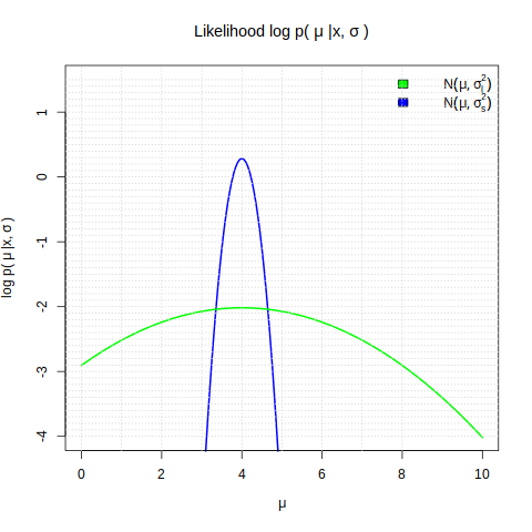
where Θ describes the distribution's scalar parameter like μ or σ in the Gaussian case. Written as vector it becomes Θ=[μ σ]. Especially in engineering it is a common case to log-transform measurements. This is for example the case in control theory or for acoustic measurements in general with the logarithmic scaled entity Decibel. The function l = log p(Θ|x) is the log likelihood. it is basically the same function p(x|Θ) but with x as fixed parameter and Θ as variable, plus the logarithmic transformation obviously. Likelihood refers to the probability for a realization x from the distribution p(x) with varying parameter Θ. The function has, instead of beeing dependent on x, the varying variable Θ and x becomes the constant parameter. As a function, it remains the same, just the variation of the parameter changes and therefore the graph might look different. The log likelihood in figure 2 below shows for that a specific value of x = 4 with varying μ. σ large is 3, whereas σ small is 0.3. With a changing μ closer to x, the logarithmic probability density arises. For the same x, just different mean value, the probablity density sinks as expected for a Gaussian. The more far from the mean, the lower the probability density.

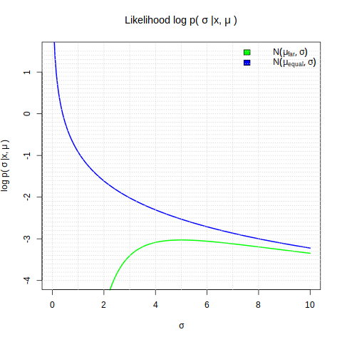
Also σ can become the variable for the log likelihood. With a fix μ and x, when already far away from mean, like the green curve where the mean is 0 and x is 3, a rising σ is not lowering the logarithmic probability density that much anymore as shown in figure 3. When σ goes to infinity, all the graphs approximate each other, as the probablity density function becomes more a constant until there is almost no mean anymore. The blue curve shows at x equal to μ=3 the logarithmic probability density sinks from infinity and approximates the common density values for large sigmas, as the density becomes very flat, almost constant for very large variances. For zero sigma, the probability has to be infinity at μ, as that value will be realized when sampled for sure. Rawly expressed, to get probability 1 for infinit small integral range, the densitiy becomes infinity. Closer x to the mean, the change of sigma is more drastic. With respect to the green curve where x is far away from mean, when sigma is very small it becomes highly unprobable that the far away x will be realized, so the log goes to minus infinity. With very small variances in that case, the probability density to realize a sample from far away from mean is highly unprobable. For large sigmas, it doesn't matter how far away the sample x from the mean μ it becomes a flat probablity density curve with more equal probablity density for all samples drawn. So depending on the region of the σ in that case, the change in probability density is different.

The smaller the sigma, the more drastic the change in likelihood (blue graph figure 3) or unlikelihood (green figure 3). Or for figure 2, the smaller sigma, the more drastic the change in the turning point on μ=x. So there is kind of a sensitivity on the probability density due to the parameter itself. Regarding figure 3, for a large variance, the dependency on μ is way stronger, as it is for a small variance. Meaning, for the same sample x, here x=4, if the μ changes, there would be a drastic drop in probability density value for the same x. Whereas, due to high variance, for the green graph, a slightly changing μ would not change that so strong. This means, for a small variance, there will be a high sensitivity on μ for the probablity density or the logarithmic probability density. That is shown in figure 4 above. Mentioning again, here it becomes seen from μ parameter, so it is called likelihood. The score function g(x) is the derivative of the log likelihood and it measures this sensitivity of the distribution to the parameter Θ in the below function as vector, with elements μ and σ. 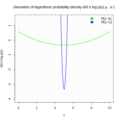As expected, at the turning point, both derivatives become essentially 0, then they arise again. 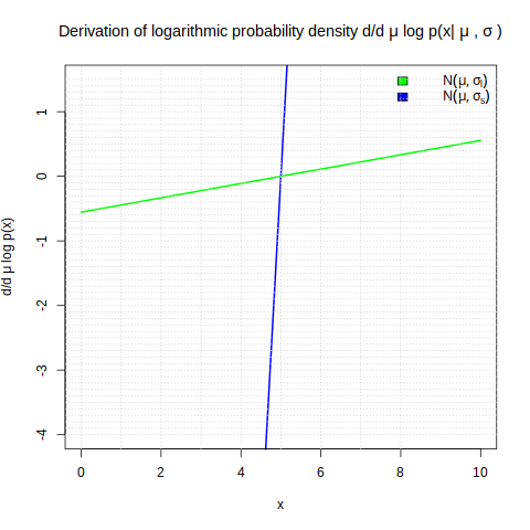Figure 4 hows the score function g(x) as a derivation by μ. The derivation arises the further away from the mean, where the derivative is 0.

The steeper the log likelihood in figure 3, the greater the value of the score function. For large variances, there is not a big change in probablity density, so the score function is expected to be small in figure 5.

The equation above for g(x) as the general formulation with the nabla operator summarizes the likelihood as dependency on either parameter, here Θ and μ.

$$$$g(x, Θ) = ∇_Θ log p(x|Θ)

The score function is the sensitivity to the parameter, here μ or σ. As there are two, they can be resembled in a matrix. The first entry would be the derivative on μ and the second one on σ. When Θ stands generally in the above function for either μ or σ, the description for the score function becomes

$$$$^d⁄_dΘ log p(x|Θ)

as simplified representation from the Nabla-Operator, which leads later to a matrix representation due to the Θ vector nature. With Θ=μ, the logarithm product rule log(a*b) = log(a) + log(b) and the potence rule log(a^b)=b log(a) the derivation becomes

$$$$^d⁄_dμ log p(x|Θ) = ^d⁄_dμ (log ¹⁄ _{√ 2πσ ²}  e^{- (x-μ)2⁄_2σ2}) $$$$= ^d⁄_dμ (log ¹⁄ _{√ 2π σ} + log e^{- (x-μ)2⁄_2σ2}) $$$$ = ^d⁄_dμ (log (√ 2π σ)^-1 + log e^{- (x-μ)2⁄_2σ2}) $$$$ =^d⁄_dμ (-log (√ 2π σ) - ^(x-μ)2⁄_2σ²)

As the first part is independent of μ only the second part remains with

$$$$^d⁄_dμ log p(x|Θ) = ^-2(x-μ)(-1)⁄_2σ² = ^(x-μ)⁄_σ²

So, either plotted over x, or plotted over μ, a constant function results in a graph like in figure 3. Plotted as x as variable, it is rising, plotted over μ it is a falling graph. On the other hand, when derivated by σ, the equation becomes The Fisher information contains therefore the score function inherently. In the Fisher information the score function is squared and from that the expectation is calculated. This is basically the formulation of the variance, here the variance of the score function. So the Fisher information is the variance of the score, which is the sensitivity of the probability density on a parameter. The Fisher information finally is the expectation of the squared of that. The above equation resembles that the expectation of E(x) is μ for a normal distribution, which we expect here. For x^2 this is μ² + σ² due to the identiy E(x²) = Var(x) + E(x)².

$$$$E_x(¹⁄_σ⁴(x-μ)²) = ¹⁄_σ⁴(E_x(x²) - 2μ E_x(x) + μ²) = ¹⁄_σ⁴ (μ² + σ² - 2μ² + μ²) = ¹⁄_σ⁴(σ²) = ¹⁄_σ²

The Fisher information is the expectation of the squared score, the sensitivity becomes only positiv for the Fisher information. with g(x, Θ) beeing a vector, g(x, Θ) * g^T(x, Θ) becomes squared and a matrix result. That is why I_x = E[g(x, Θ) * g^T(x, Θ)] as a (2x1) x (1x2) matrix becomes a (2x2) matrix with the diagonal elements beeing the squared scores. That is how the score vector for a normal distribution becomes g(x, Θ) * g^T(x, Θ) = [ ^d⁄_dμln N(x|μ, Θ^2); ^d⁄_d&Theta^2;ln N(x|μ, Θ^2) ] with partial derivatives.

But for the Fisher information the square of that result is needed before its integration. So the intermediate result becomes:

$$$$(^d⁄_dμ log p(x|Θ))² = ¹⁄_σ⁴ (x-μ)²

With a larger σ, the flatter the curve and the smaller the Fisher information. μ only shifts the curves vertically. To calculate the Fisher information, this intermediate result multiplied by p(x) is integrated to get the expectation of the intermediate result samples. With a changing μ, p(x) shifts equally.

$$$$ ℑ_x = ∫_x ¹⁄ _{√ 2πσ ²}  e^{- (x-μ)2⁄_2σ2 1}⁄_σ⁴ (x-μ)² dx

Sensor takes a lot of measurements. Let the expectation be Gaussian distributed. If you like to know mean value. How much information the samples of a distribution contain about the distribution's parameter. Gaussian A sample has more information content about the mean of Gaussian distribution when the variance is smaller. Score function is derivative of log likelihood.

The p11 Element of the Fisherinformation matrix is the derivation on μ of the squared score function. It remains independent of μ and therefore, the Fisherinformation remains only dependent on σ not matter what μ it is. This is intuitive, as the mean value only shifts the curve vertically.

One could ask why all the effort to estimate covariance matrices. But common measurement correlation is used for example with the Information Matrix Fusion algorithm (IMF) for sensor fusion. Sensor fusion often uses Kalman-Filters to estimate the target through multiple sensors. The Kalman-Filter algorithm applies the process covariance and the measurement covariance. The fusion of measurements from multiple sensors is highly applied in autonomous driving also because of redundancy.

When sampling from a sensor, like a Radar sensor in autonomous cars that measures horizontal distance x in centimeters as event, it would be necessary to know the amount of information that an observated sample carries about the μ and σ of that measure x. If it was the task to estimate those values from samples, it would be great to know how much information each sample carries about those parameters. The more information a sample contains, the better to estimate. This information is called the Fisher information.

[1] Wikipedia: Béziere curve

The Fisher information then is defined as:

$$$$ ℑ_x = 𝔼[(^d⁄_dΘ log p(x|Θ))²] = 𝔼[l'(x|Θ)²]

The expectation of the squared score function for a probability density, where the score function is the derivation of the log likelihood for a probablity density function.